# Properties of issuance level (part 1) 1\. In my [last thread](https://notes.ethereum.org/@anderselowsson/MinimumViableIssuance), minimum viable issuance was introduced as an important guideline for staking economics. This thread will take a closer look at how issuance level affects Ethereum’s equilibrium staking conditions and guide us toward a utility-maximizing reward curve. 2\. This thread is also available on [Twitter](https://x.com/weboftrees/status/1745043778262421544) and [Farcaster](https://warpcast.com/anderselowsson/0xb289e9ae), and I will shortly provide an ethresearch post covering the topic for those more comfortable with that format. Part 2 is also in preparation. 3\. Before I start I would like to thank Barnabé Monnot, Francesco D’Amato, Vitalik Buterin, Thomas Thiery and Justin Drake for fruitful discussions and feedback for this thread, as well as Ansgar Dietrichs, Davide Crapis, Caspar Schwarz-Schilling and Julian Ma for fruitful discussions. I also wish to thank [Flashbots](https://www.flashbots.net/) for providing the data used for this analysis. --- 4\. The demand curve shifted upwards after The Merge when stakers started to receive MEV and priority fees. Reservation yields fell after Shapella due to improved liquidity, and the supply curve shifted downwards. Both changes pushed up the equilibrium quantity of stake. 5\. Because of this, Ethereum has arguably entered a phase of overpaying for security. To what extent can we stop overpaying? Can we reduce issuance while still retaining consensus stability, proper incentives, and acceptable conditions for solo staking? 6\. Can we adopt a reward curve that lets the issuance yield go negative past some specific staking deposit size $D$, or target some specific desirable $D$ by simply adapting the yield to enforce it? Otherwise, should a more moderate approach be adopted? 7\. We will take a closer look at these questions and review features of staking economics that affect consensus incentives and reward variability—including how they vary across deposit size. This will guide our approach to minimum viable issuance (MVI). ## Relationship between the equilibrium staking and $F$ 8\. The base reward factor $F$ is the big knob for adjusting the total issuance level under the current reward curve. It affects all consensus rewards and penalties and provides an issuance yield under idealized performance of $y_i = \frac{cF}{\sqrt{D}}$, where the constant $c\approx2.6$. 9\. The total yield provided by the protocol to stakers implies its demand for stake and it is $y=y_i+y_v$, where $y_v$ is the yield from realized extractable value (REV). Denote yearly REV as $V$ (currently around 300k ETH). We then have $y_v=V/D$. 10\. Note that $y$ is the "[endogenous yield](https://x.com/weboftrees/status/1710720809797407063?s=20)" derived exclusively from staked participation in the consensus process. The yield from DeFi/restaking that is exogenous to staking is not modeled here; it can under competitive equilibrium also be derived by non-stakers. 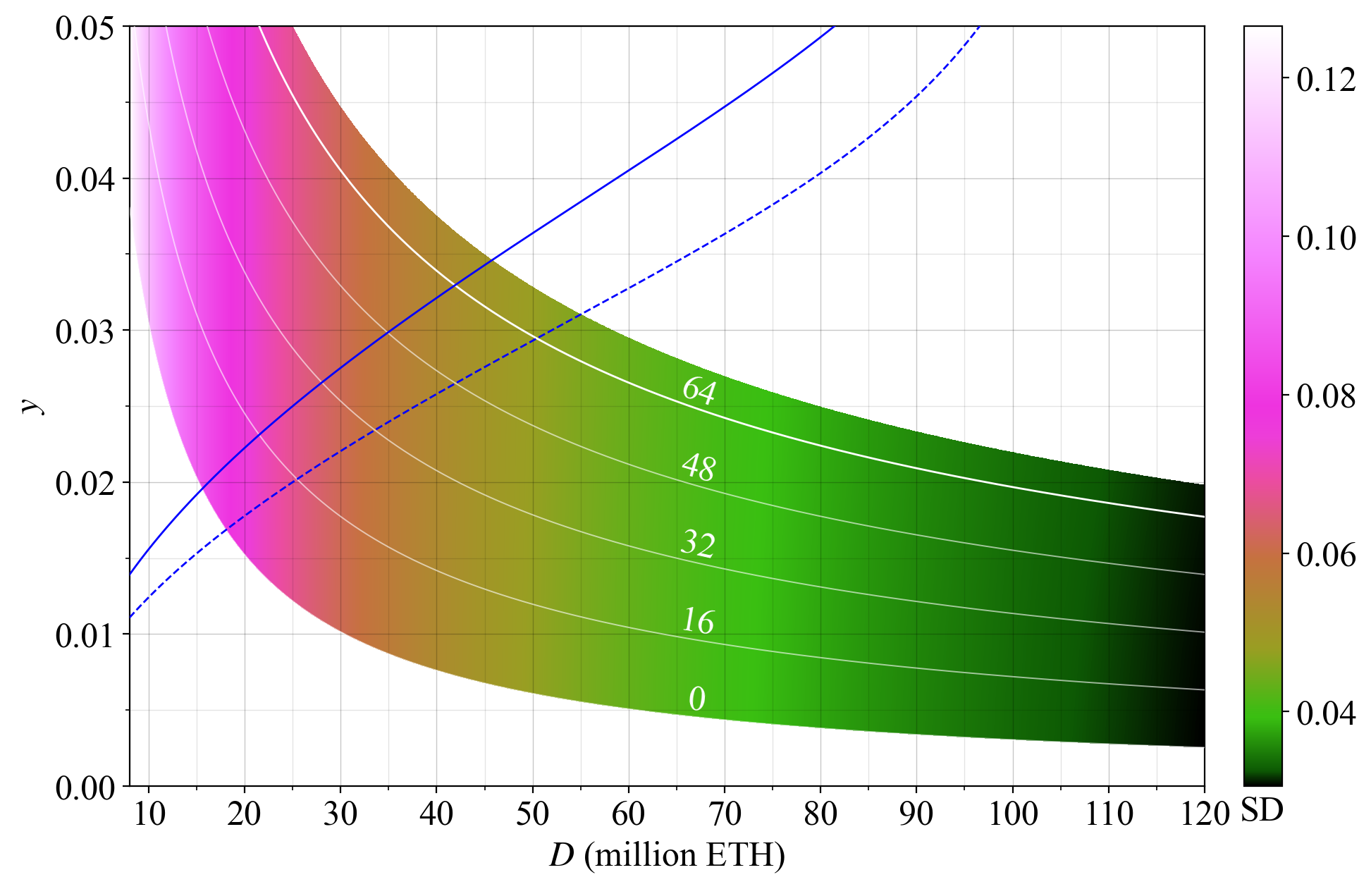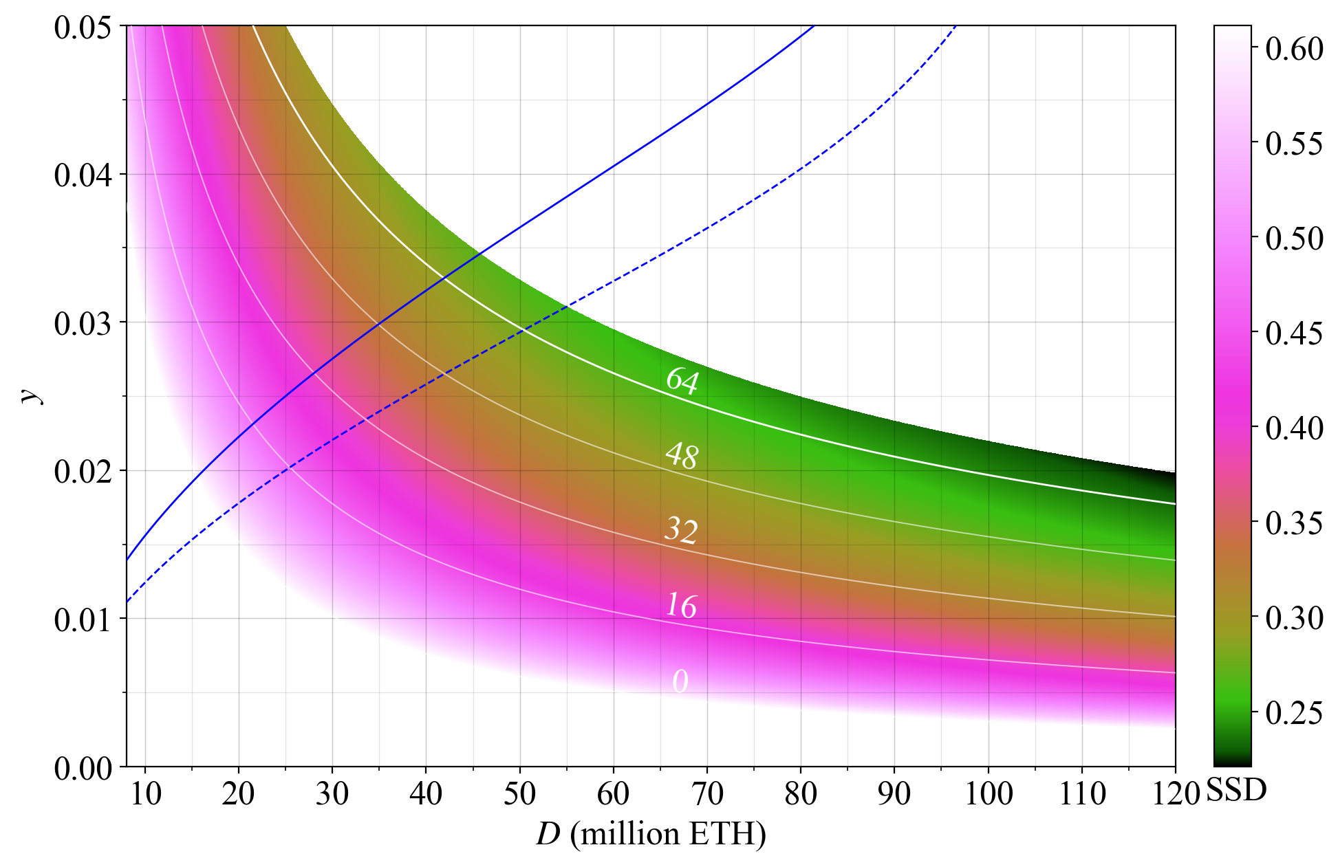11\. The colormap and y-axis both capture $y$, with the colormap restricted to $F \in [0, 75]$. Currently, $F=64$. At equilibrium, the demand curve will intersect the supply curve that [captures](https://x.com/weboftrees/status/1710705504320684087) how prospective ETH holders’ inclination to stake varies with yield.  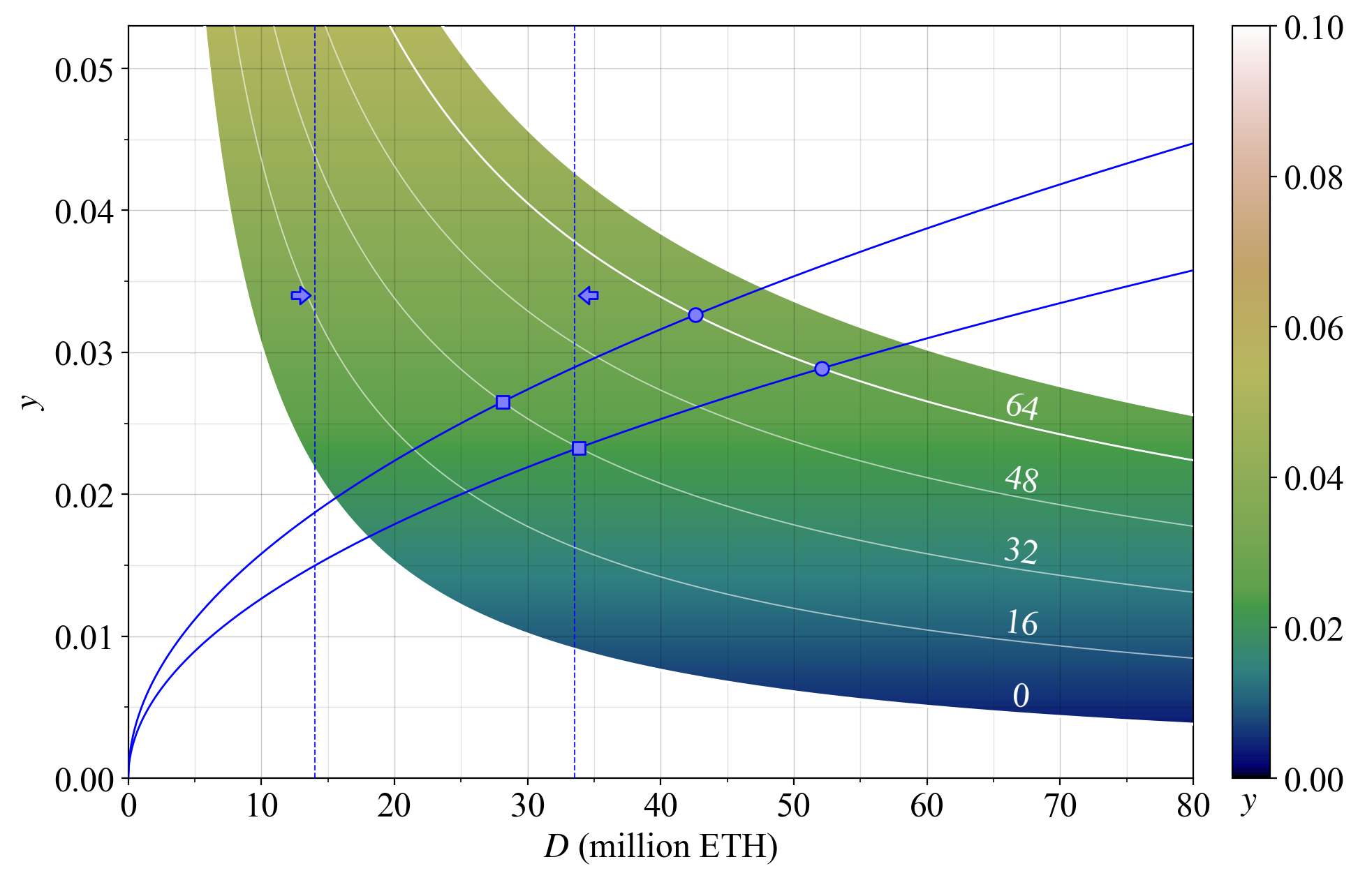12\. The shape of the supply curve is unknown. The two examples in blue have a yield elasticity of supply of 2, with the lower also used in the [last thread](https://x.com/weboftrees/status/1710706011185545671?s=20). Plots will be provided covering a broader range so that different assumptions can be mapped to various outcomes. 13\. The upper curve could for example represent the supply curve underpinning a medium-run equilibrium (within a year or two), whereas the lower curve could be the supply curve after a few years of improvements to the the staking experience and better financial integrations. 14\. The left dashed blue line indicates the revealed preference of The Merge at $D=\,$ 14M ETH. By staying to the right of this line, we are operating at a deposit size that has been [previously regarded as sufficiently safe](https://x.com/weboftrees/status/1710717027520831749?s=20) by the Ethereum community. 15\. The right dashed line indicates $2^{25}$ ETH (33.6M ETH), which has been [used](https://notes.ethereum.org/@vbuterin/single_slot_finality) as a reference point capturing when network conditions (and economics) start to degrade. By staying to the left of the line, Ethereum is better positioned on these issues. 16\. Potential equilibria under the current issuance policy ($F=64$) and REV are indicated by blue circles, and the equilibria if issuance is halved ($F=32$) are indicated by blue squares. Such a reduction brings the deposit size closer to a previously suggested desirable range. 17\. It is not possible to ascertain the exact effect of a reduction in $F$, but we can be rather certain that the yield elasticity of supply for the medium run is not 0 (a vertical supply curve). Reducing $F$ will therefore always reduce the quantity of stake, ceteris paribus. 18\. Note that the full reduction in yield from a change in $F$ (white downwards arrow) will not remain at the new equilibrium, because some stakers will presumably leave (blue leftwards arrow), bringing the yield for remaining stakers back up a bit (white leftwards arrow).  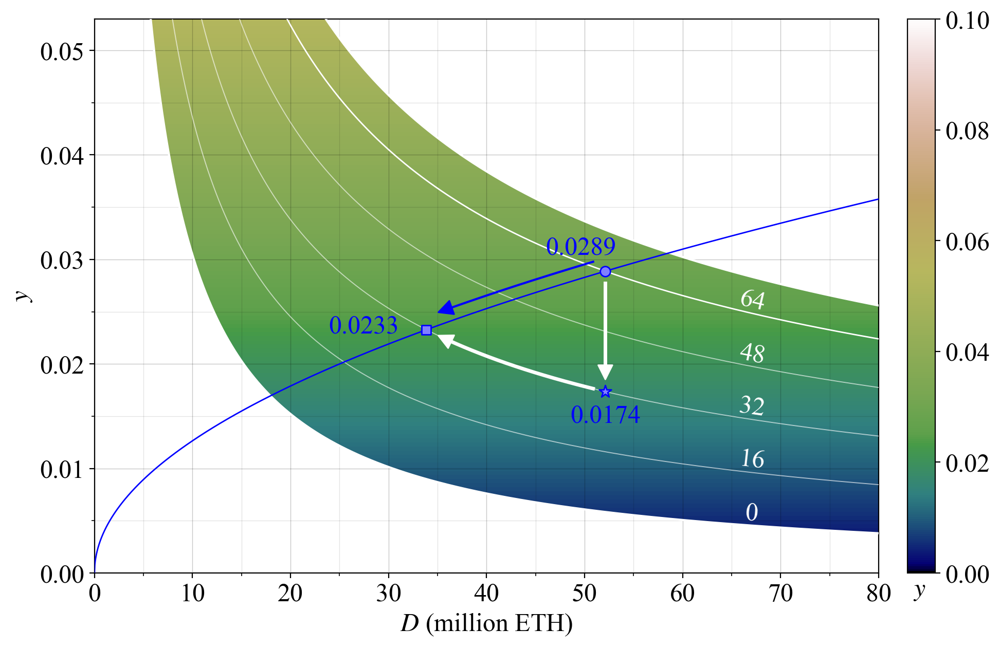19\. For the specified supply and demand curves, the equilibrium yield initially falls from 2.89 % to 1.74 % when reducing $F$ from 64 to 32 (a reduction of around 2/5), but then comes back up to 2.33 % as some stakers leave. The equilibrium yield is thus reduced by around 1/5. 20\. How will this dynamic affect the solo staker and delegating staker? The outcome over shorter time horizons will depend on variations in cost structures and frictions affecting the decision to stake or de-stake. 21\. A solo staker who will not buy new hardware at some low yield may still stake over the lifetime of their current hardware. Delegating stakers dissatisfied with the yield may keep their savings in the LST until the next time they wish to spend their money, or leave directly. 22\. Solo stakers’ upfront costs and illiquidity [presumably](https://x.com/weboftrees/status/1710719952968106177?s=20) give them a lower yield elasticity of supply in the short run. This is comforting, because a temporarily lower-than-equilibrium yield (if $F$ is reduced in a hard fork) may not push them out forever. 23\. It seems likely that the supply curve will gradually shift downwards over time as the staking experience simplifies and DeFi integrations improve. The outlined dynamic in §18 may therefore not fully materialize, as a lowering supply curve can nullify any de-staking process. 24\. The equilibrium quantity of stake will however still be lower with a reduction in $F$ than if $F$ is kept fixed. We must evaluate each possible outcome at the medium-run equilibrium. The effect of a gradually lowering supply curve is a gradually increasing deposit size/ratio. 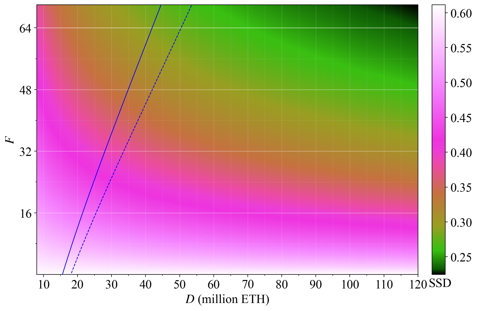25\. This figure has $F$ on the y-axis instead of yield. You may think of it as dragging down and straightening the bent colormap in §11 such that it becomes a rectangle. The colors encode the same yield as previously (also indicated by black lines).  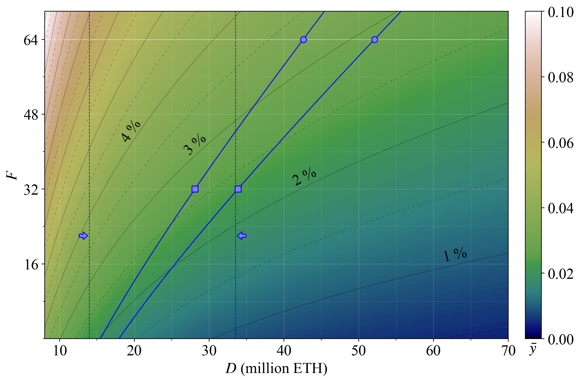26\. This viewpoint is convenient as we will now further explore the effect of a change to the issuance level. We will often provide both alternative graphs to the reader and indicate the same two supply curves as guidelines. ## Incentive structure 27\. When contemplating a change to the issuance policy, it is important to consider the effects on consensus stability, in particular how incentives may change for different consensus roles that validators will be assigned to. 28\. This figure shows the expected rewards stemming from issuance at various settings for the base reward factor $F$. The hypothetical equilibria are once again indicated. Naturally, the lower $F$ is set, the lower the proportion of rewards that come from issuance.  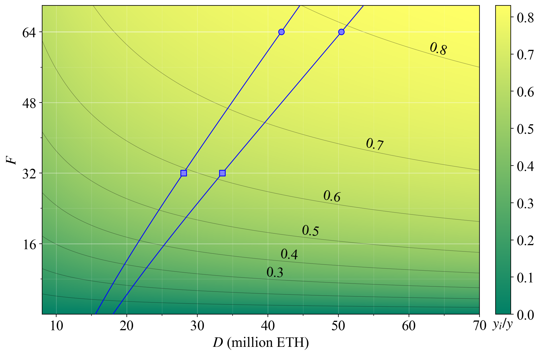29\. Right now at the prevailing level of REV, more than 2/3 of rewards come from issuance. Since $y_v$ falls by the reciprocal of $D$, whereas $y_i$ falls by the reciprocal of $\sqrt{D}$ under the current reward curve, a higher proportion of rewards will stem from issuance at a higher $D$. 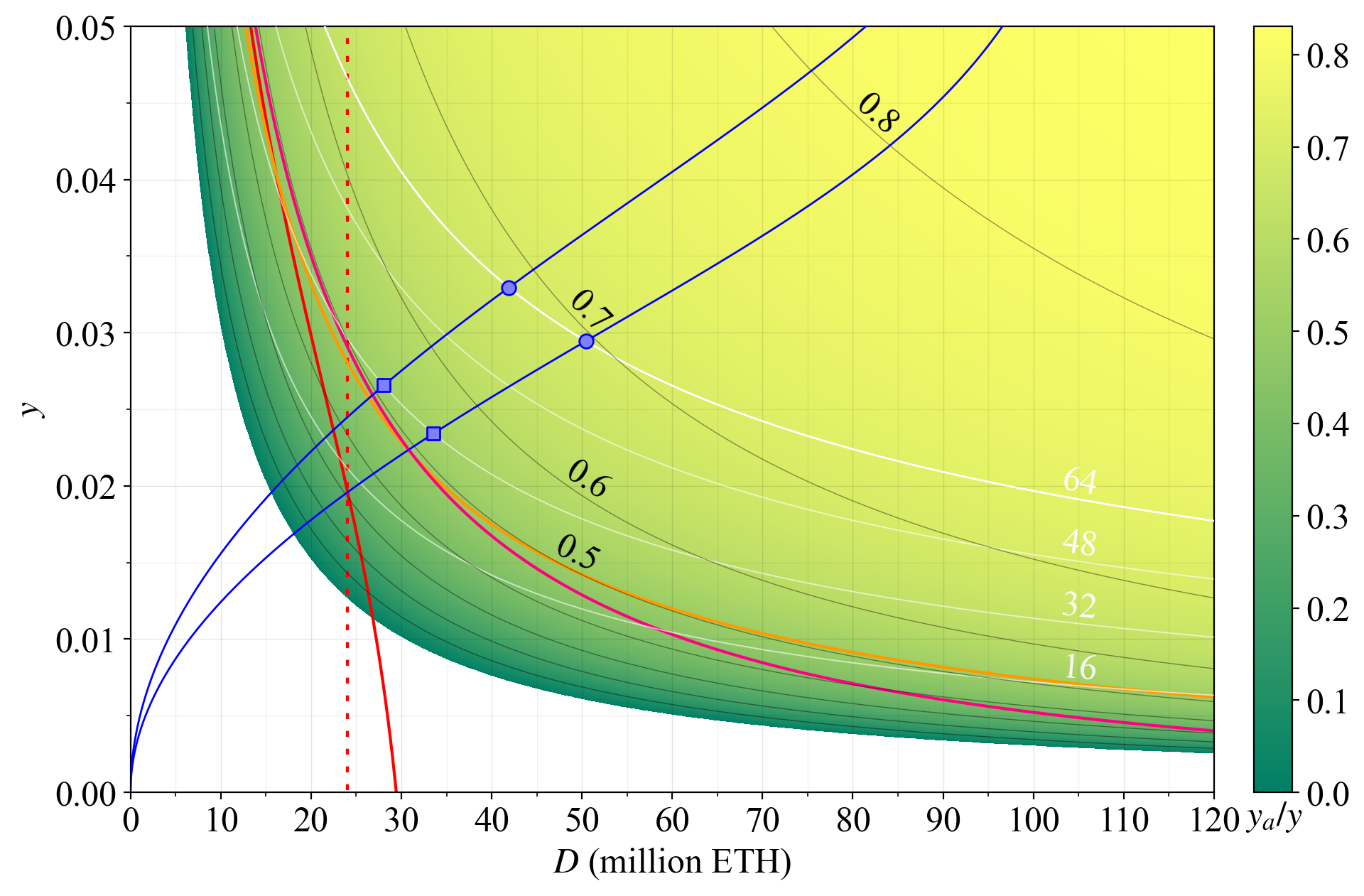30\. This figure instead shows the yield that comes from attester duties ($y_a$) in proportion to the total yield ($y_a/y$). Since the proposer gets 1/8 of the issued rewards, the situation under this viewpoint worsens somewhat.  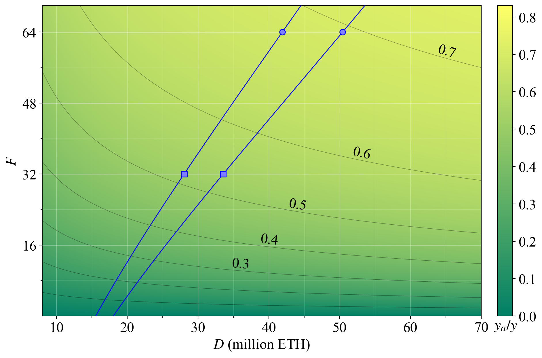31\. If $F$ is reduced to 32, almost half the rewards will come from the sparse chances of proposing a block. There is no well-defined proportion of $y$ that must be provided for attester duties, but higher is generally better, and providing at least 0.5 for them seems healthy to me. 32\. When $y_i/y$ and $y_a/y$ fall too low, the consensus mechanism breaks down. Consensus rewards and penalties stop providing correct incentives for stakers. Honest attestation is less compelling. The only thing that matters is to collect REV and to not get slashed. 33\. Ignoring attester duties comes at little to no cost as long as the inactivity leak is not triggered, and instigating reorgs will be more tempting. If REV rises relative to the proposer reward, timing games also become a little more attractive. 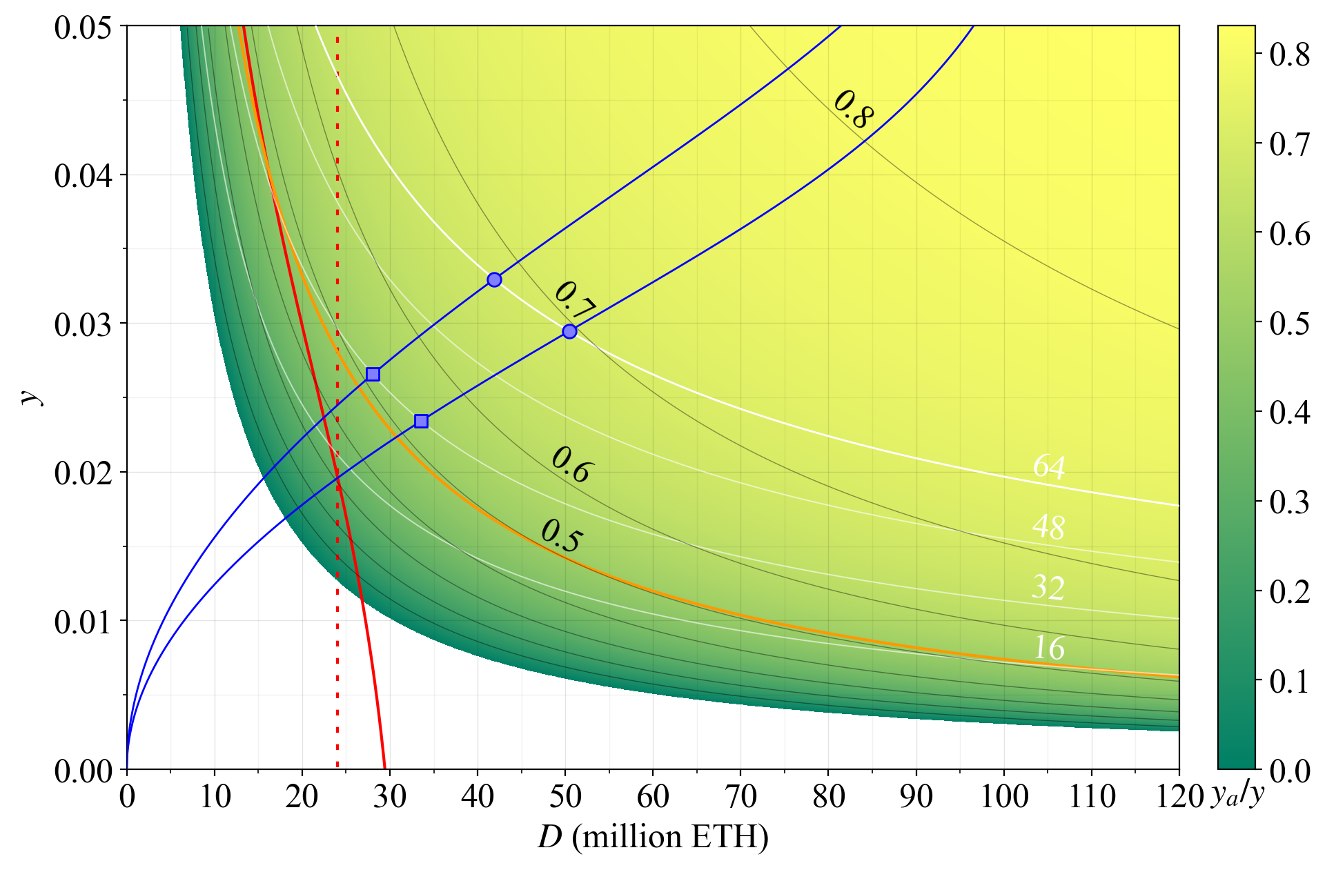34\. Moving back to having staking yield on the y-axis gives another perspective on how various hypothetical changes to issuance policy may affect the proportion of rewards awarded for attestation duties. This time, the x-axis extends across the full circulating supply.  35\. In red, we contemplate the various stricter issuance policies that can be attempted, and the adverse effects they may bring before MEV burn is in place. For example, to target $D =\,$ 24M ETH (dashed red line) while keeping $y_a/y>0.5$, the yield must be around 3 % (red square). 36\. This seems unreasonably high given that the supply curve slopes upwards. Therefore, to enforce $D =\,$ 24M ETH, an even lower proportion of rewards must be given for attester duties. Indeed, it may not be possible to give these duties any issuance rewards at all (i.e., 0 issuance). 37\. Such an outcome is manifested by an equilibrium in the white region of the figure. This could be the outcome if the supply curve over time drifts lower---which seems like a very reasonable assumption---or simply because of a not particularly unlikely rise in REV. 38\. The same type of problem can be encountered when adopting a reward curve that goes negative to enforce a deposit size below some specific level. The red line indicates the reward curve [previously suggested](https://notes.ethereum.org/@vbuterin/single_slot_finality) by Buterin. 39\. At many reasonable equilibria with such strict reward curves, the rewards for attester duties will be very low (red circles), or non-existent. The breakdown in accordance with §32-33 is then complete. 40\. Note that the supply curves in the last three figures were adjusted slightly to illustrate the notion that the final fraction of the circulating supply would not be staked in the medium run until the yield becomes very high. The equation is $y=c_1d^k + \frac{c_2d}{1-d}$, using the deposit ratio $d$ (the fraction of circulating ETH that is staked), with $k=1/2$ (a yield elasticity of 2), $c_2=0.003$, and $c_1$ set as [described](https://x.com/weboftrees/status/1710706011185545671) in the last thread. --- 41\. As previously outlined, when $D$ rises, the white region representing $y_v$ becomes smaller and smaller. This happens because $y_v$ falls by the reciprocal with a rise in $D$. I highlight this because it is currently not very well understood. 42\. For example, as a motivation for “EIP-7514: Add Max Epoch Churn Limit”, it is implied that $y_v$ could be “much higher” than $y_i =$ 1.6 % at 120M ETH staked, but this is unreasonable. At the prevailing level of REV, the expected $y_v$ would be just 0.25 % at 120M ETH staked.  --- 43\. Some of the issues of a lower issuance here outlined can be remedied by taking out a staking fee each epoch and increasing the base reward correspondingly. To prevent consensus breakdown, the fee must be introduced already at positive yields. 44\. However, introducing a fee challenges long-standing tenets promoted to solo stakers ("you can go offline X % of the time and still break even", etc.). Trying to push through these far-reaching changes when MEV burn eventually can make them obsolete therefore seems undesirable. 45\. Furthermore, a staking fee will not resolve other issues of a very low issuance, such as a rise in the relative and equilibrium variability in rewards for stakers that do not pool their MEV income. ## Variability in rewards for solo stakers 46\. The variability in rewards is higher for solo stakers than delegating stakers under the current consensus mechanism, because delegating stakers can in a frictionless manner rely on pooling of rewards from a large number of validators. This affects solo stakers negatively. 47\. A change in issuance policy could further widen the gap in variability, and it is therefore necessary to model that. The most prominent research on reward variability has been done by [@pintail](https://twitter.com/pintail_xyz), with [analysis](https://pintail.xyz/) up until and just after The Merge. 48\. The reader is also encouraged to study writings on [this matter](https://eth2book.info/capella/part2/incentives/rewards/#individual-validator-rewards-vary) by [Edgington](https://twitter.com/benjaminion_xyz). In fact, the whole chapter on the incentive layer is fundamental reading to any consensus layer developer. 49\. This thread models variability for solo validators over one year in a rather simple fashion, with the distribution in proposer and sync-committee duties assigned according to the probabilities given from the consensus spec at each modeled deposit size. 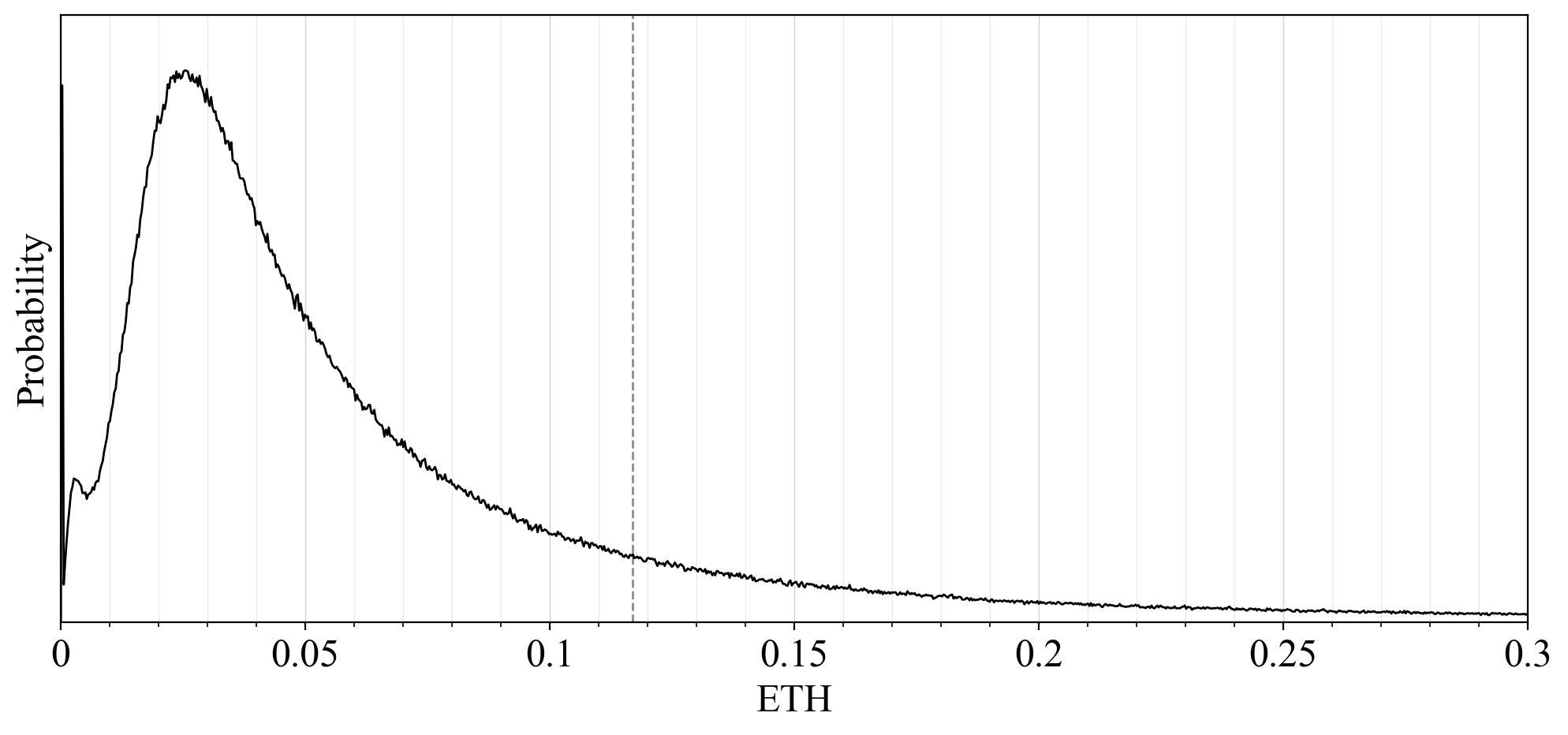50\. The focus is on the greatest source of variability, namely that of variation in REV. To this end, block proposers are assigned REV using sampling with replacement from the roughly 2.7 million block-level sample points [provided by Flashbots](https://flashbots-data.s3.us-east-2.amazonaws.com/index.html). 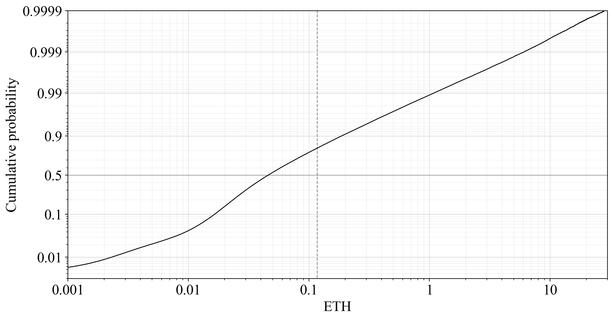51\. A probability density function (PDF) of the REV in Ethereum shows a positive skew, with a mode of around 0.025. The mean of around 0.12, indicated by a dashed vertical line, is higher due to the occasional blocks with very high MEV.  52\. To discern more details, the cumulative distribution function (CDF) is here plotted with a log-scaled x-axis and a logit-scaled y-axis. The median MEV is around 0.045 ETH and less than 20 % of the slots are above the mean. Note the occasional >10 ETH outcome.  53\. Blocks have been missed with a probability of around 0.96 % since The Merge, a condition that is also included in the model. Missed sync-committee assignments are not precisely modeled and instead assigned to have the same probability as missed blocks. 54\. It is presumably less common to fully miss the sync-committee assignment (which spans over more than a day), and much more likely to partially miss it, but modeling this exactly is beyond the scope of this thread. 55\. Notably, blocks are to a higher [proportion](https://x.com/nero_eth/status/1742534075343061363?s=20) missed by solo stakers than professional stakers, something that further degrades conditions for solo stakers when $y_i$ is reduced relative to $y_v$. This specific feature is not included in the model. 56\. Finally, attesters are assumed to perform their duties correctly and are set to receive the full rewards (a slight overestimate). Attestations will produce much less variability that is out of the control of the operator than block proposals, so they are less relevant to this analysis. ### Effect of pooling 57\. The figure plots the influence of pooling on CDFs of yield at the current deposit size of $D=29$M ETH. Annualized validator rewards were simulated 30M times, sampling REV with replacement (s. w. r.). Pools were created from these distributions, also s. w. r. 30M times.  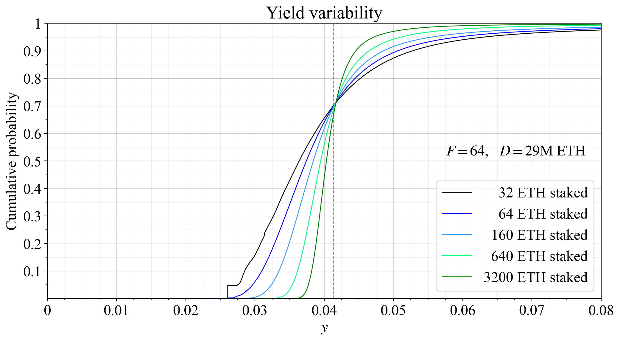58\. As evident, variability is gradually reduced with more staked ETH (the curve becomes steeper). A solo staker running 2 or 5 validators can already reduce variance quite a bit; a small pool managing a couple of thousand ETH will still not be able to fully remove variance; etc. 59\. We are not mainly focused on variability in the present, but rather at the medium-run staking equilibrium. The focus is to investigate what kind of variability that can be expected under different supply and demand curves. 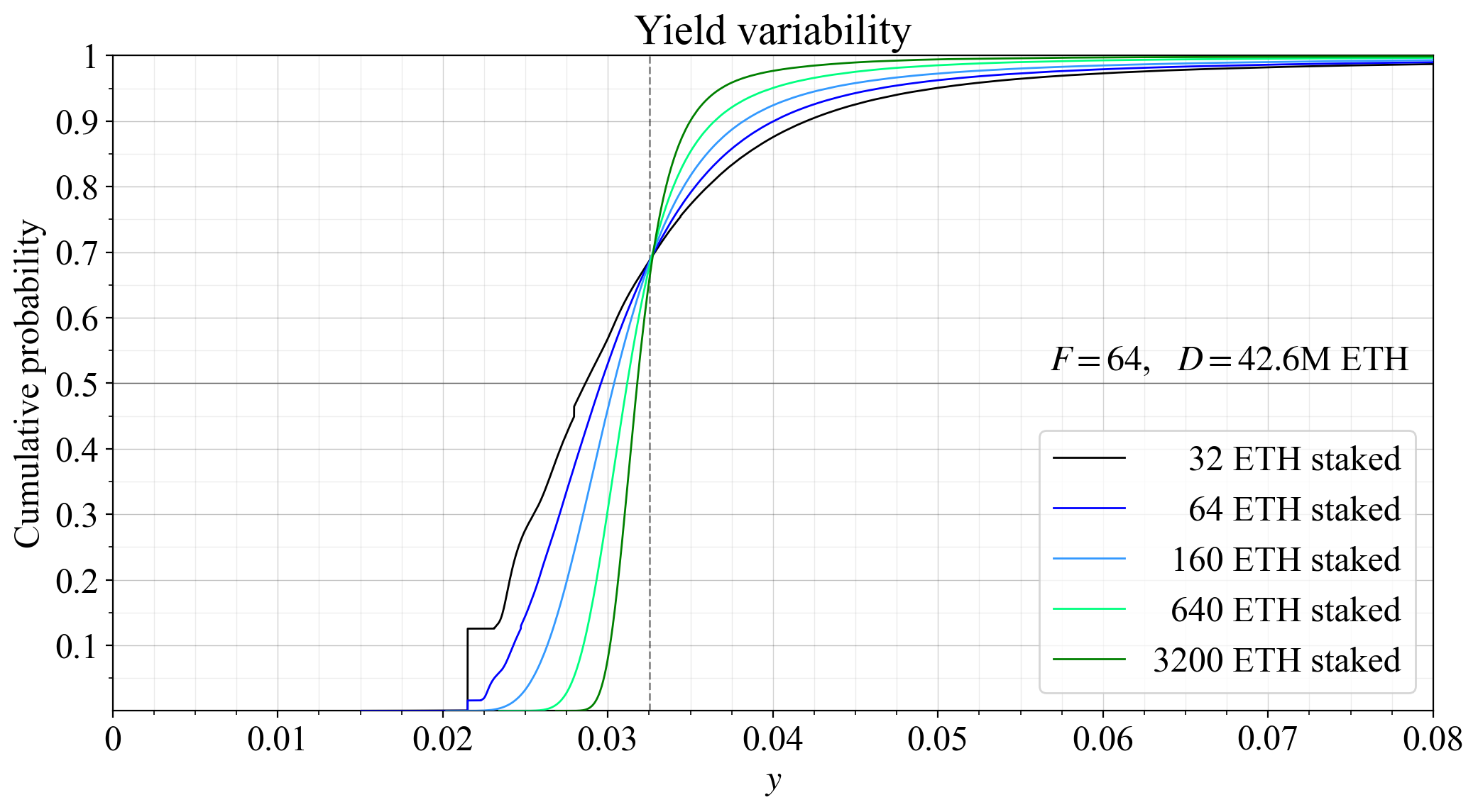60\. With the higher supply curve from previous plots, the equilibrium staking is around 42.6M ETH. The figure shows the variability under such a deposit size, otherwise using the same conditions as previously. Average $y$ (indicated by a grey dashed line) falls at the equilibrium.  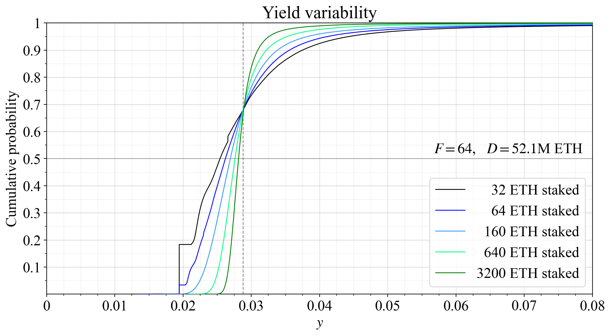61\. With the lower supply curve, the equilibrium is $D=\,$ 52.1M ETH, as here plotted. The vertical part of the black line, representing solo stakers with no block or sync-committee assignments, is now rather noticeable. It consists only of attestation rewards (idealized performance).  ### Variability with fixed supply and varied demand 62\. We now take a look at how variability in yield changes for solo stakers when $F$ is changed. The plot shows the equilibrium CDF under the lower supply curve (the average is dashed). When $F=0$, only MEV remains, and stakers with no block proposals receive no rewards at all.  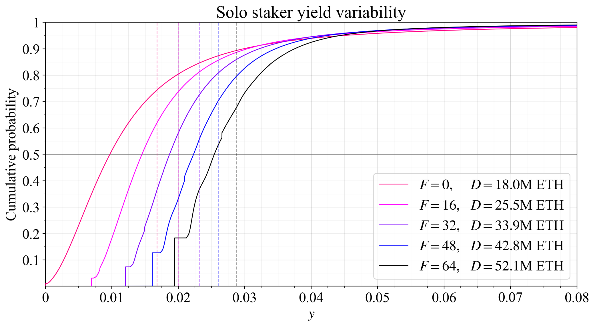63\. To better illustrate the risk solo stakers take on in comparison with delegating stakers, all cumulative probability distributions were normalized by subtracting the average yield (“shift-normalized”). This preserves the standard deviation (SD) of each distribution.  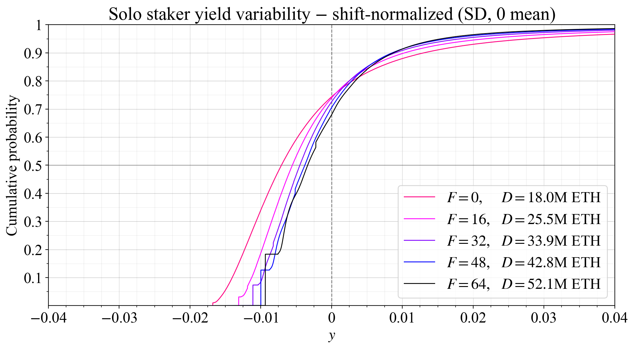64\. It is now easier to observe how a change to $F$ increases variability at the medium-run equilibrium. The effect is particularly prominent at $F=0$, and also noticeable at $F=16$. From $F=32$ and above, the increase in variability relative to $F=64$ is less significant. 65\. The SD is illustrative when discussing how the shape of the distribution affects risks. But the SD (or variance) is insufficient for capturing the full impact of variability for the risk-averse staker. The higher-order moments of the distribution also matter. 66\. In particular, a positive skew is favorable. In this regard, Ethereum’s yield distribution is certainly better than its inverse, where there would be a small risk of losing everything. The worst-case scenario for honest and attentive stakers is thus an important feature. 67\. Solo stakers may in reality be worse affected at the same SD when the expected yield is lower. As a simplified example, say that solo stakers are some fixed proportion of all stakers at any deposit size when there is no variability in rewards, and that the supply curve rises linearly. 68\. Then, if the expected yield is 2 % and can vary uniformly between 1-3 %, half of the solo stakers would need to account for the risk of receiving a yield below their reservation yield over a year. If the expected yield is 5 % but can vary between 4-6 %, the proportion affected is 1/5. 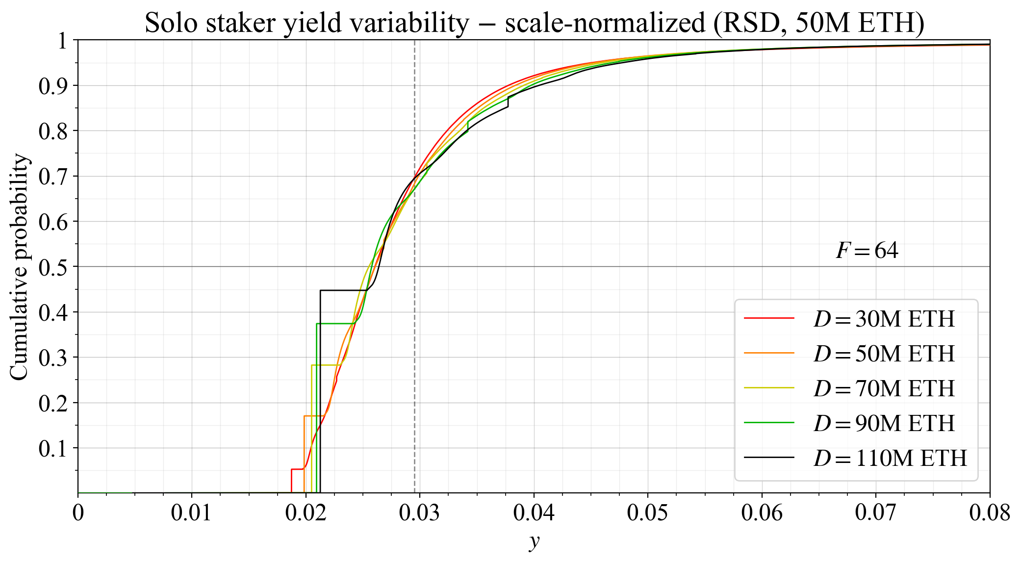69\. This figure accounts for such relative effects, instead normalizing by dividing each distribution by the ratio between its mean and the mean at $F=64$ (“scale-normalized”). This preserves the relative standard deviation (RSD) of the distribution (computed as SD/mean yield).  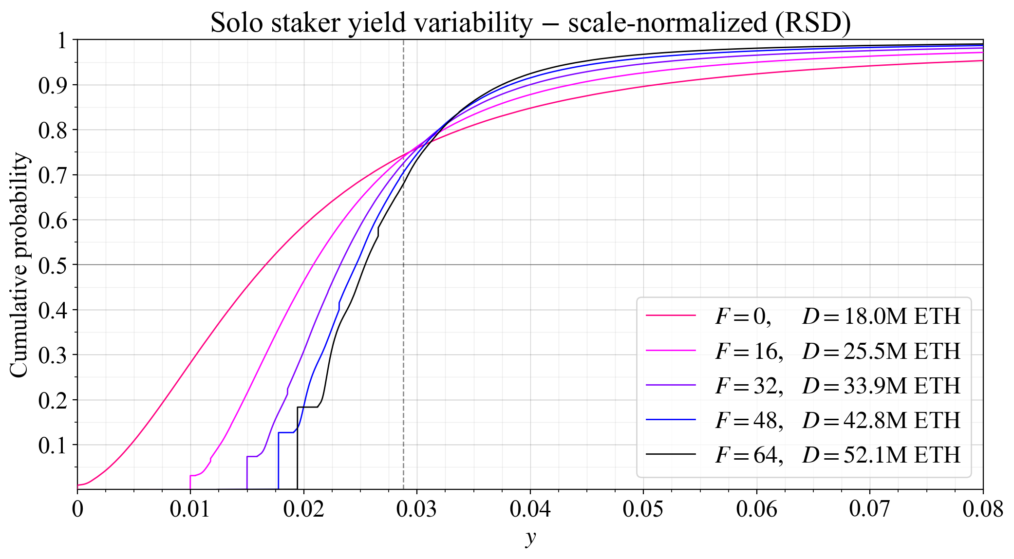70\. From such a perspective, variability for solo stakers certainly starts to degrade already around $F=32$, and more so at $F=16$. But this is just one viewpoint on the matter, both the SD and RSD convey something important about the solo stakers’ conditions. ### Variability with fixed demand and varied supply 71\. Another interesting perspective is to vary $D$ while keeping the reward curve fixed, thus computing variability across demand. This allows us to study equilibrium distributions, where each one is the result of a different supply curve. 72\. From a consensus developer’s perspective, this is a very important viewpoint and will be the focus going forward in this thread. As developers, we can control the shape of the demand curve (particularly after MEV burn), but cannot materially alter the supply curve. 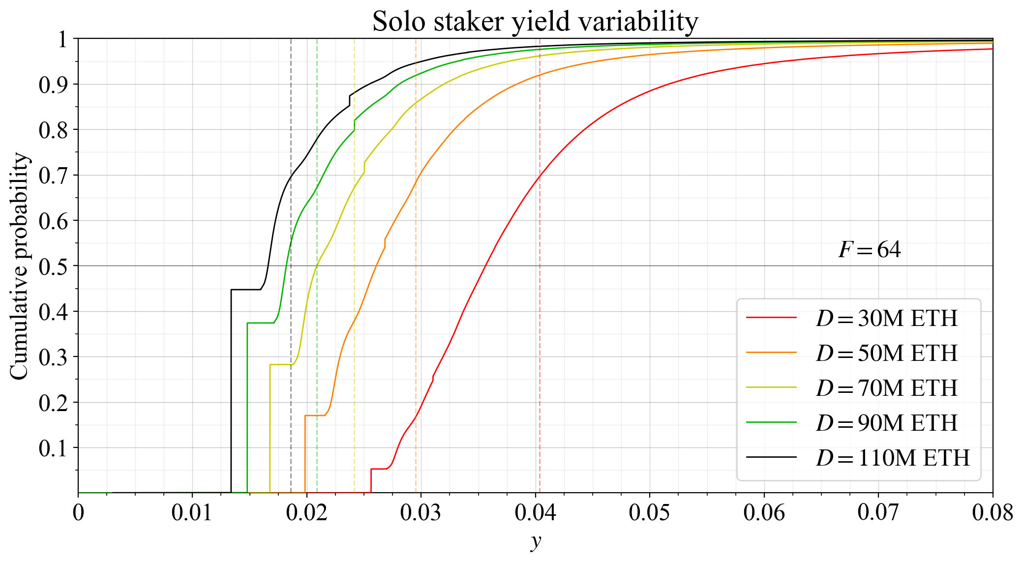73\. This plot shows CDFs across the current reward curve. In the very unlikely case that the marginal staker at 110M ETH staked has a reservation yield below 2%, almost half the validators will neither propose blocks nor sync-attest over the year at equilibrium (vertical black line segment).  74\. Still, as implied by the shift-normalized distributions, the SD *decreases* with an increase in deposit size, keeping $F$ fixed. This may be surprising to some given that the rarity in getting selected for special duties increases.  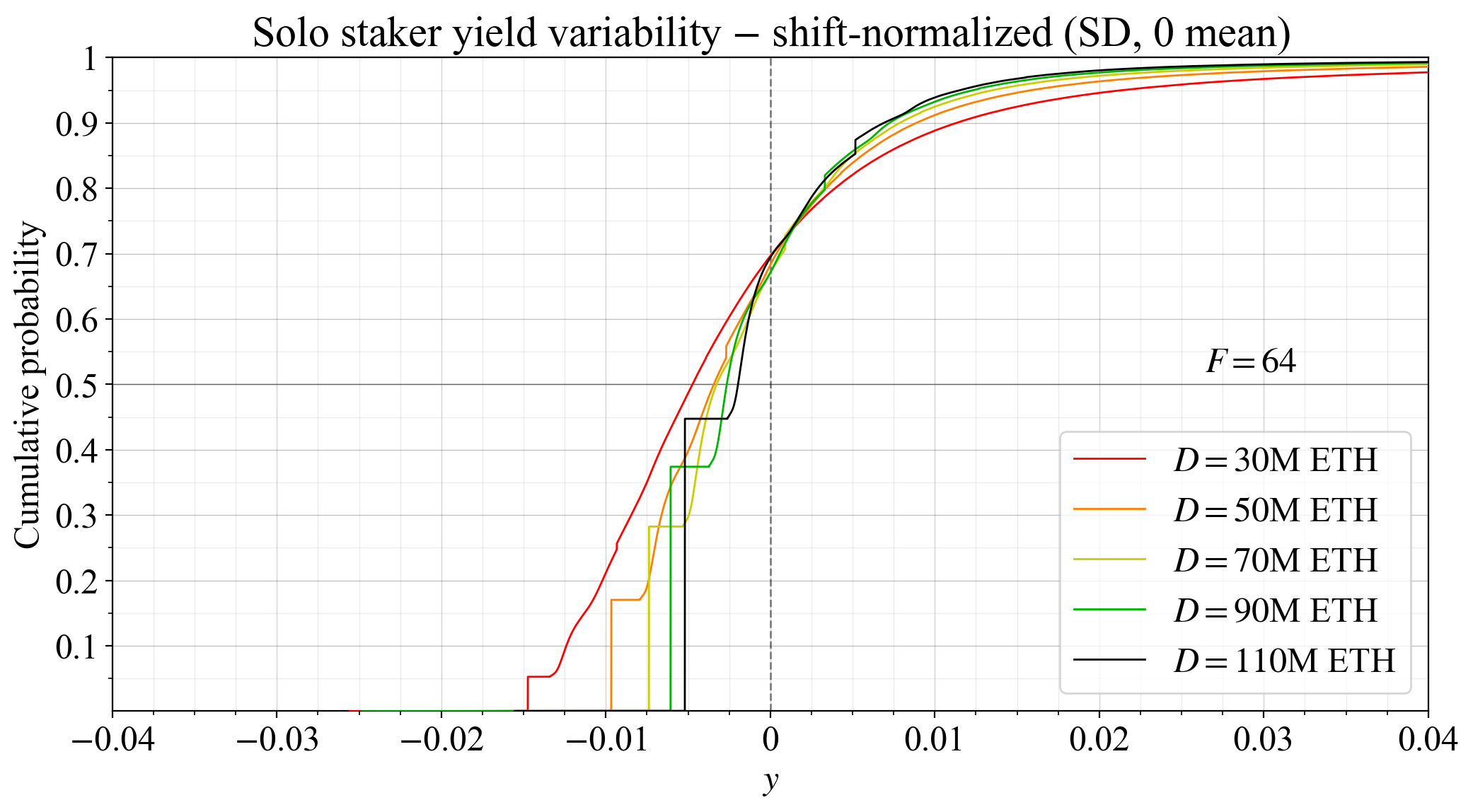75\. But a validator having been selected one time to propose a block will not be put on hold to let other validators take their turn; such a solution would not work. Also remember that the standard deviation is computed after first subtracting the mean. 76\. When it comes to the RSD, it is kept relatively fixed across $D$ under the medium-run equilibrium, as indicated by the scale-normalized figure. This is opposed to the SD which is more or less fixed across $F$ at the same $D$.  77\. If $F$ is reduced to 32, the equilibrium deposit size will fall. We ignore this and plot the distributions at the same fixed $D$ as previously. The yield at 110M ETH staked is then just above 1%, and the unlucky solo stakers with no assignment only receive around 0.7 %.  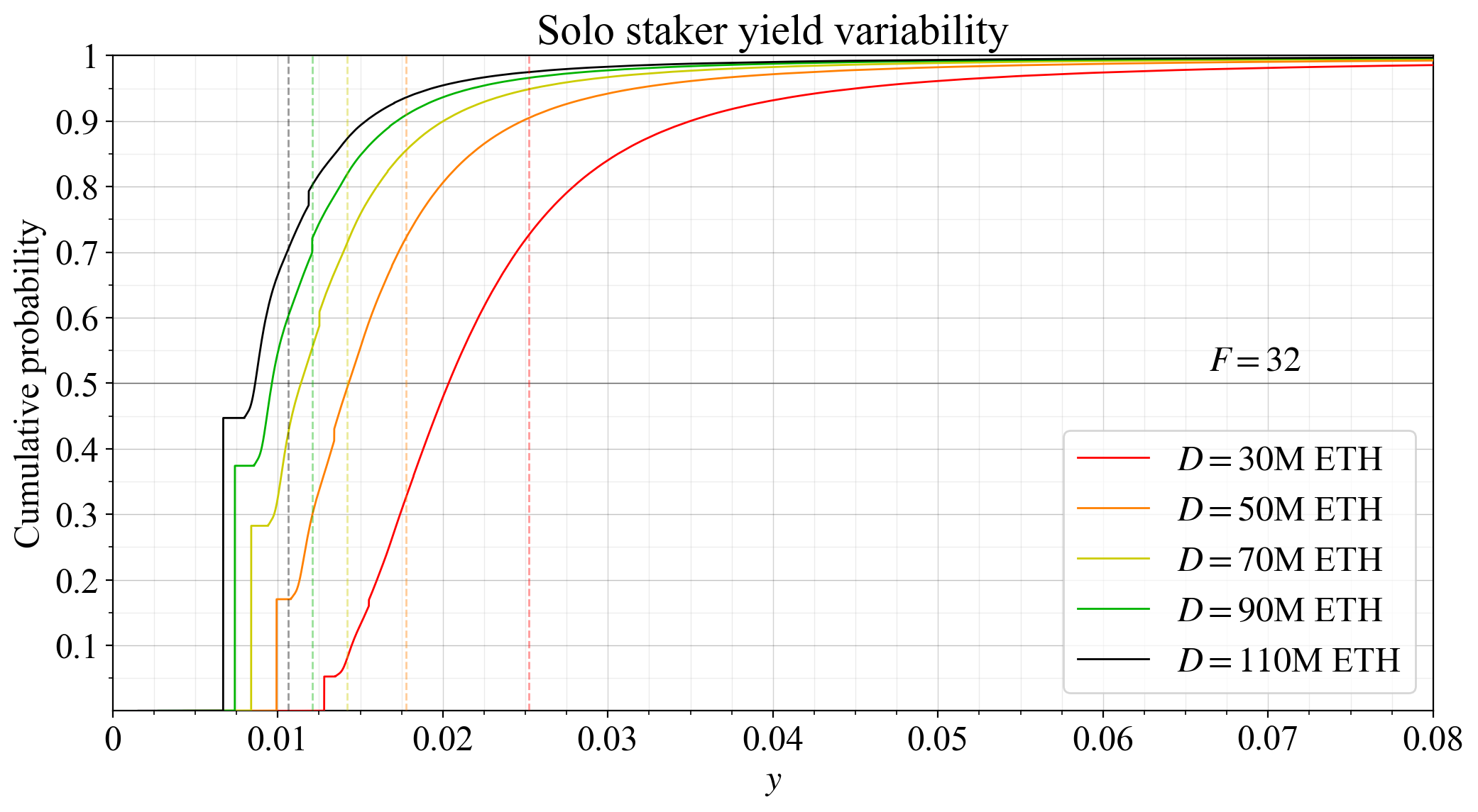## Two-dimensional mappings of solo-rewards variability 78\. It is now time to map the previously investigated variabilities across two dimensions, to provide a better understanding of the influence of variability on Ethereum staking economics. 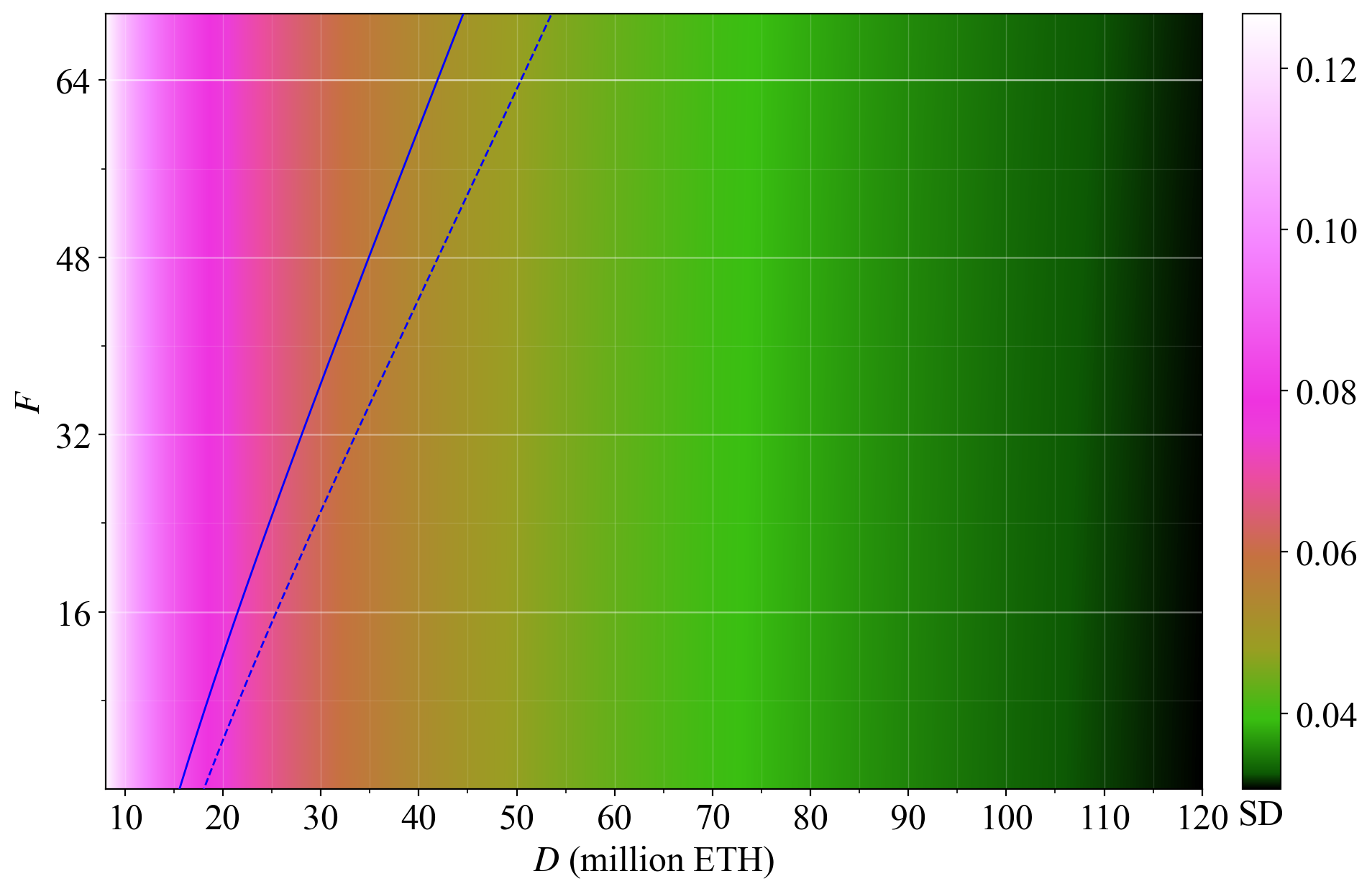79\. The mappings were done by simulating solo staker's yearly yield 70M times (sampling REV with replacement), repeated across $10^5$ different deposit sizes and across 32 different settings for $F$. Smoothing was applied (across variance) and upsampling performed across $F$. 80\. The first figure shows how the SD varies across $D$ (all the way up to 120M ETH) and $F$. A lower SD is better. The base reward factor has but a minuscule effect on the SD at any specific deposit size, because issuance level shifts the yield rather equally for everyone.  81\. The same outcome can be observed with total endogenous staking yield on the y-axis. To produce this graphical representation, the simulated outcome from the previous plot was simply interpolated onto the new axes. One supply curve is dashed for easier connection to the next plot.  82\. Since the quantity of stake supplied increases with a higher yield, the reality is that a higher $F$ will produce a lower standard deviation in rewards under equilibrium. This figure captures the equilibrium SD across $F$ for the two modeled supply curves (equilibria for the lower are dashed).  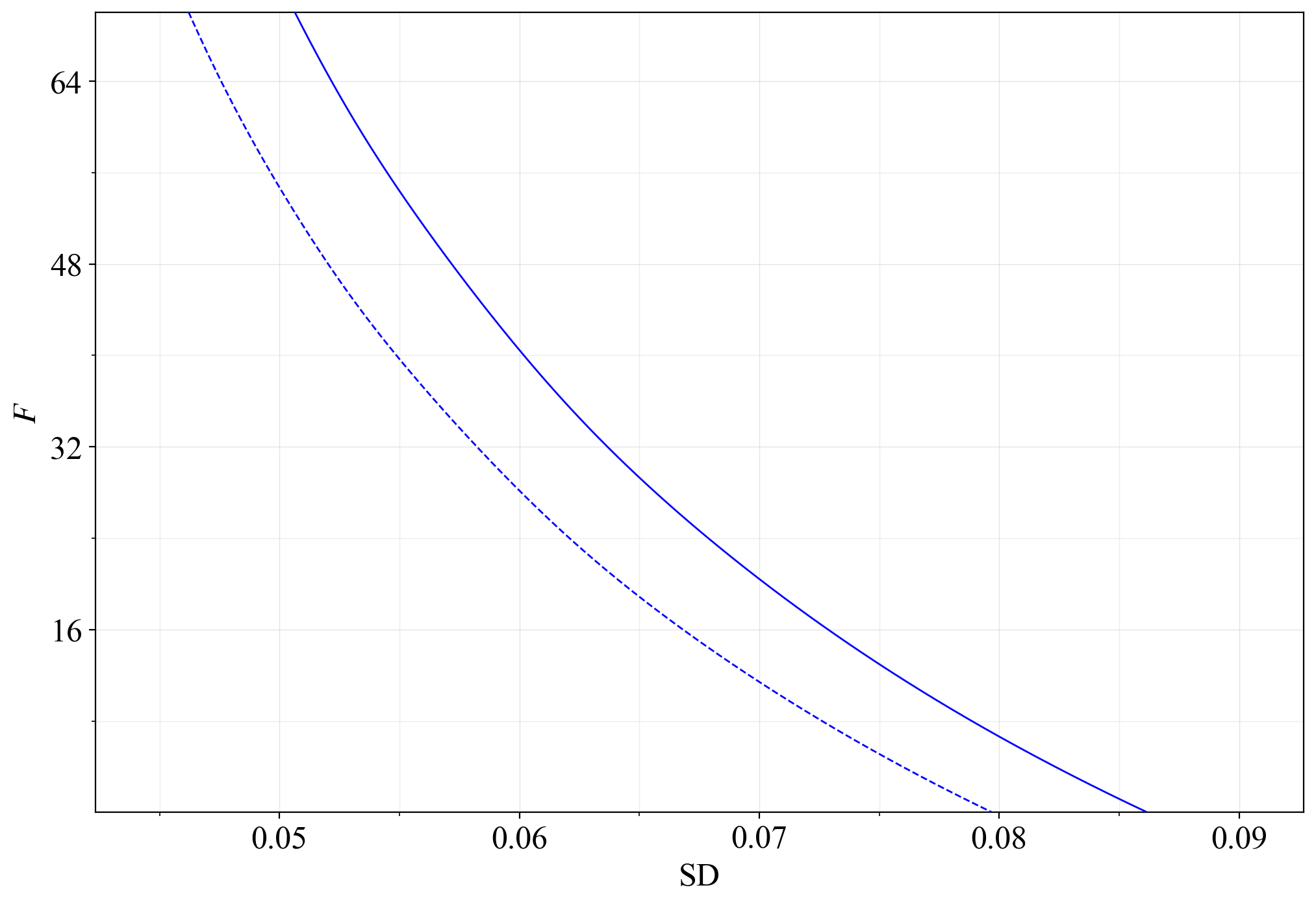83\. Thus under these assumptions, lowering $F$ will indeed increase the equilibrium variability for solo staker while MEV burn is not in place. But the increase at 48 or even 32 is rather modest. 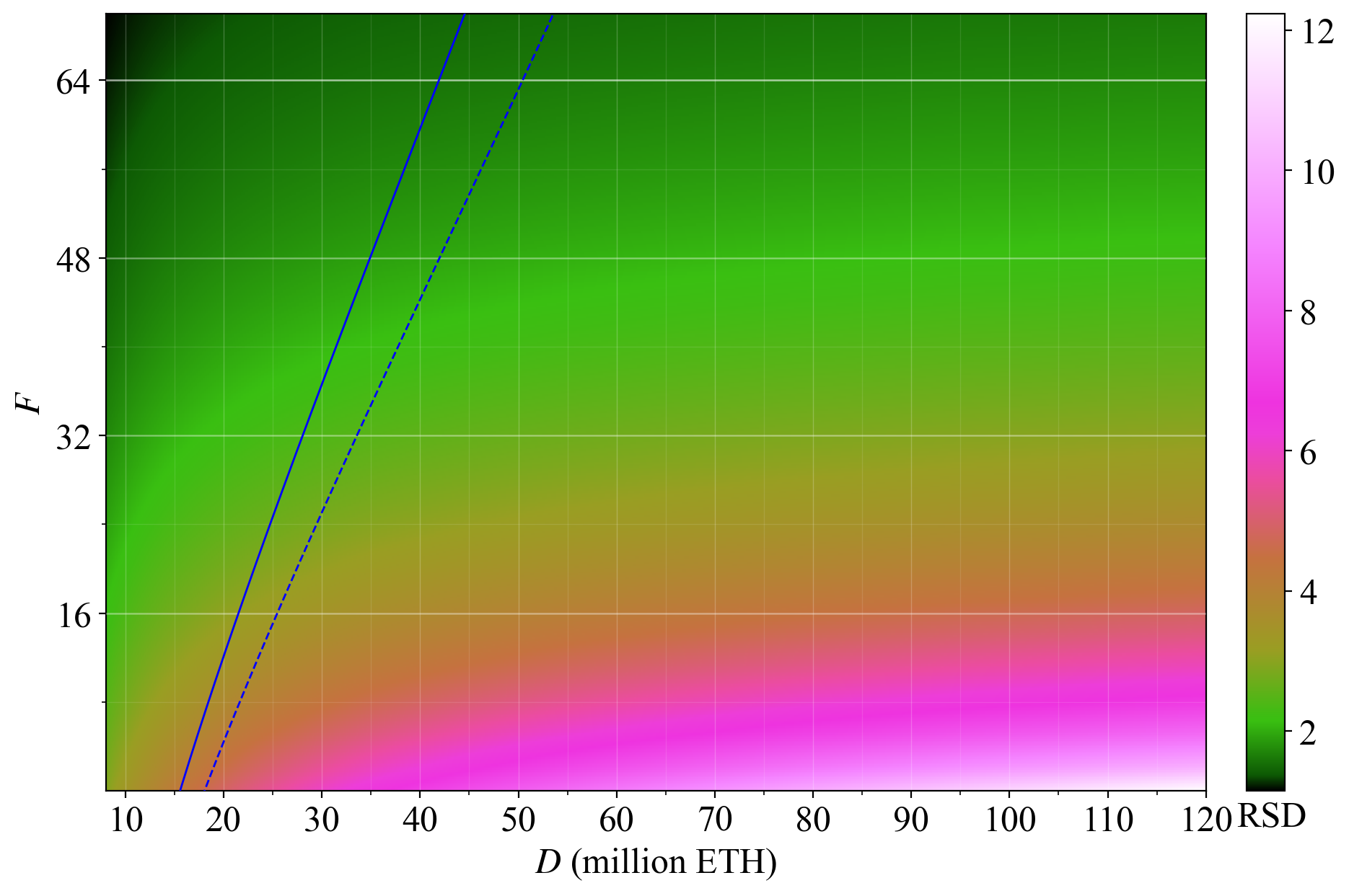84\. Recall that another interesting perspective is the relative standard deviation (RSD), which captures the notion that a high standard deviation can be worse at a lower yield than at a higher yield. The RSD is here depicted across $F$ and $D$ (lower is better).  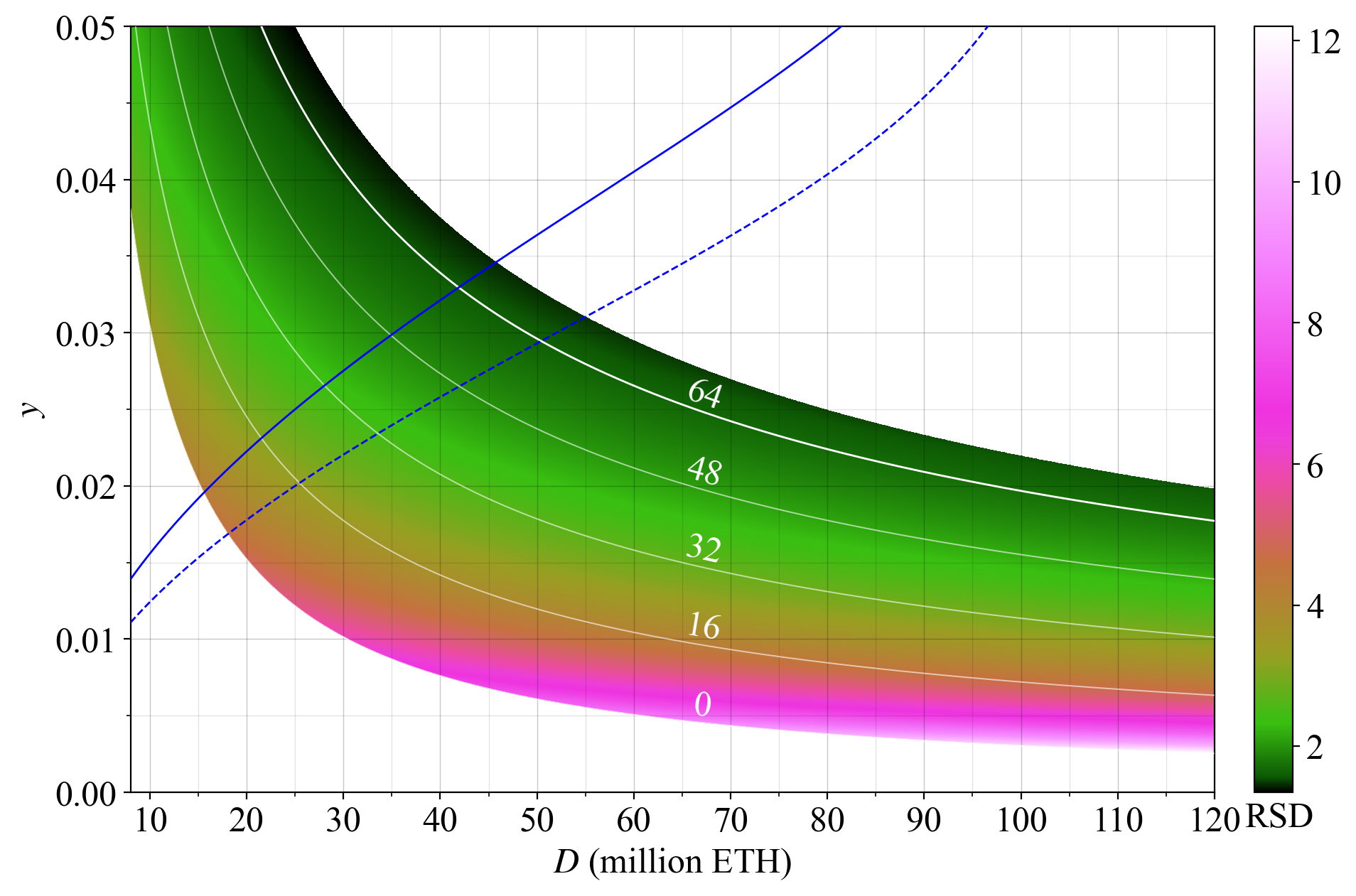85\. This figure instead captures the RSD across $y$ and $D$. When going by the RSD, a higher $F$ is clearly preferable, because it serves to push up yield in general, thus facilitating a higher equilibrium yield and lower RSD.  86\. Arguably, the SD puts too much emphasis on variabilty and the RSD puts too much emphasis on the mean. Therefore, some measure in between these two seems appropriate for further modeling. Define the SSD as the standard deviation divided by the square root of the mean. 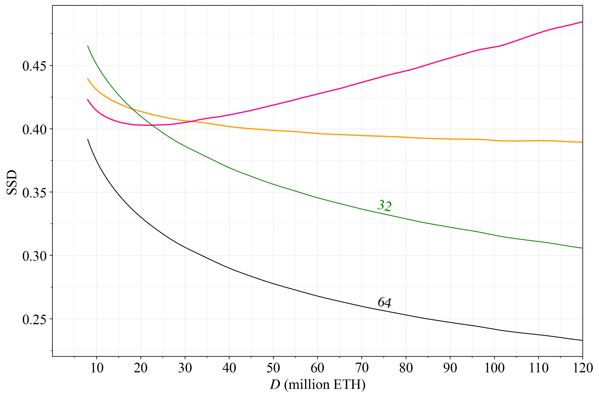87\. These figures plot the SSD (lower is better). Under the combined measure, if $F$ is kept fixed, a staking equilibrium at a higher $D$ gives a lower SSD. To make the issuance policy more “neutral”, the reward curve can be designed to produce the same SSD under any supply curve.   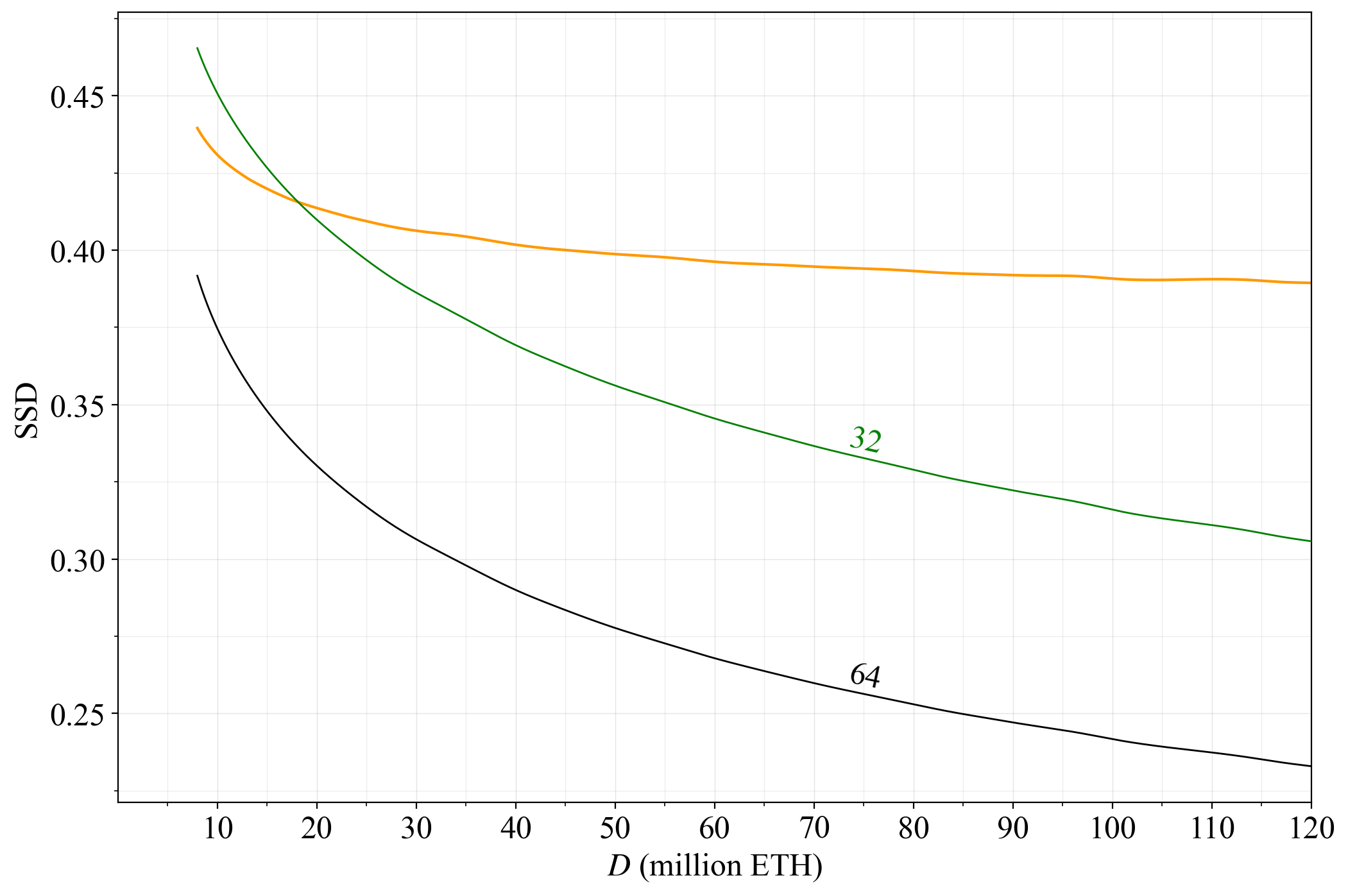## Towards a utility-maximizing reward curve 88\. How then can a more “neutral” issuance policy, specifically a more neutral reward curve be constructed? This figure plots the SSD across the reward curves with $F=32$ and $F=64$. In orange is a more neutral reward curve, preserving a set SSD at any equilibrium.  89\. This reward curve is also neutral across $D$ concerning the proportion or rewards awarded to attesters, as shown here in the familiar plot against the attester proportion with $y$ and $D$ on the axes. It ensures that attestations will bring in around half of the yield at any deposit size.  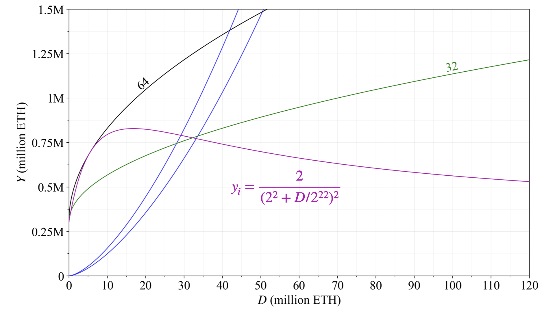90\. Its equation for the issuance level is the log-logistic $\frac{c\,\sqrt{D}}{2^{11}+\sqrt{D}}$ with the scaling constant $c$ used for setting a desirable asymptotic maximum issuance. In these figures, $c=2^{19}$ ETH, but this is just the minimum that ensures $y_a/y\approx0.5$, and can be raised. 91\. The reward curve will asymptotically approach a negated inverse issuance-yield elasticity of demand of 1. That measure generalizes the parameter “$p$” of the current reward curve $cFD^{-p}$ with $p=0.5$. I have [long been in favor of a “$p$-elasticity” of 1](https://x.com/weboftrees/status/1615200349207560192?s=20) for moderating yield. 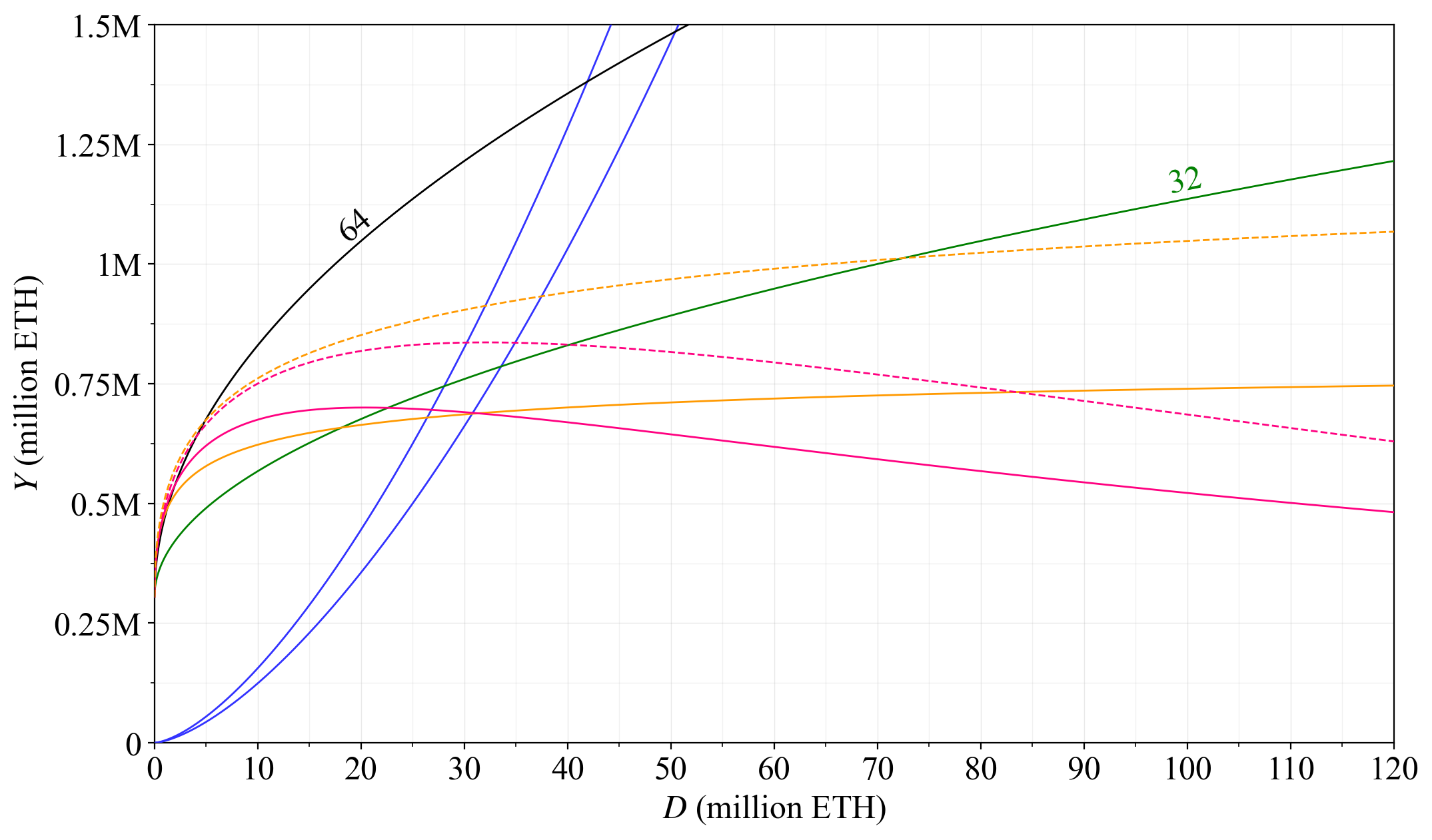92\. When plotting the total yearly distributed rewards $Y$, it is easier to see that the presented reward curve in orange will also still provide better guarantees for preserving a staking level above the revealed preference of 14M ETH than when relying on $F=32$.  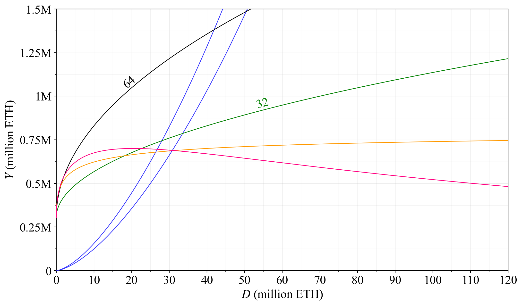93\. If even more certainty is desired regarding this feature, the scale parameter set to $2^{11}$ could be reduced slightly, or the asymptotic issuance level of $2^{19}$ raised. Indeed, simply keeping issuance fixed at $2^{19}$---removing the reward curve completely---would likely work rather fine. 94\. The orange curve achieves some form of neutrality in terms of variability and consensus balance. It implies that we are willing to sacrifice the same level of utility degradation in these features whatever the deposit size is. But we may not actually want such neutrality. 95\. The pink curve illustrates a less neutral alternative. Its equation for the issuance level is $\frac{\sqrt{D}}{2^{13}+\sqrt{D}}-\frac{D}{2^{27}+D}$ and the expression is also scaled as needed by multiplication with a constant, here $11^6$. 96\. With such a reward curve, yield provided for attestations can become less than half of the total yield at higher deposit sizes, as here illustrated. It expresses that some utility degradation from consensus imbalance is acceptable to temper utility degradation from a high $D$.  97\. There is of course also a probabilistic component to this analysis: the level of REV is not fixed and no specific proportion of rewards for attestation duties can be guaranteed. In the scenarios where the equilibrium $D$ is higher, it is more likely that REV is also higher. 98\. The SSD for solo stakers goes up a little at higher deposit sizes with the pink less neutral reward curve. But as suggested previously, this may be acceptable.  --- 99\. Another aspect is the [minimum yield under which solo staking](https://x.com/weboftrees/status/1710720252462428628?s=20) on an efficient setup is feasible. The protocol facilitates 32 ETH solo validators and should thus ensure that $y$ covers their minimum operational costs. Other outcomes seem pathological. 100\. Such considerations add weight to a maintained/rising issuance above around 70M ETH, and may push us closer to the orange than the pink curve---ultimately depending on ETH-denominated hardware cost. These aspects will be discussed in part 2 of this analysis. --- 101\. It may be easier to find agreement on something closer to the dashed reward curves formed by multiplying all variables of the solid curves by 2. A middle ground that can be implemented under rough consensus is better than the status quo.  102\. This includes a middle ground of settling the base reward factor higher than $F=32$, say $F=40$ or $F=48$. Such a change would still be helpful---albeit a little less so---with the understanding that MEV burn is still in the cards and will naturally affect staking rewards as well. ## Conclusion and discussion 103\. It is important to recognize the need for formulating our issuance policy as derived from a set of tangible utility measures, providing a rationale for its implementation. Each deposit size can be assigned a maximum protocol utility issuance level. 104\. In the absence of a consensus redesign and/or introduction of a staking fee, that level is never too close to 0. But it is also important to not let issuance go above what is needed for retaining security---because that degrades utility for users. 105\. In a world without MEV or concern for the conditions of solo staking, designing our issuance policy would be a simpler affair. But MEV will imbalance consensus roles, produce variability, increase uncertainty and keep us from achieving MVI until we burn it. 106\. If we succeed in burning MEV, a staking fee will presumably not be needed. If the total endogenous yield is zero or negative, there are no direct incentives for staking. It will then [be better to "restake" WETH](https://x.com/weboftrees/status/1710724981326279033). Implementing a staking fee thus seems hard to motivate. 107\. While the protocol could allow information about the implied supply curve to influence issuance in the future (i.e., autonomous adjustments), such practices are currently not very beneficial when contemplating our strict dependency on MEV. 108\. Still, the impetus for tempering our issuance policy should be clear from my thread on MVI. It is of course not desirable to incentivize users to stake when there is no need for it. The options thus available to us can essentially be divided into three categories: | Description | Analytical overview | | -------- | -------- | | A reduction of the base reward factor, keeping the current reward curve. | The change is minimal and easy to overview and implement. However, the current reward curve specifies an increasing issuance even as the deposit size rises far above what is needed for security, and therefore does not facilitate MVI. | | A reward curve that approaches constant issuance. | Issuance is maintained at the same level relative to MEV, ceteris paribus. This keeps several important features rather neutral across $D$. Acts as a middle ground. | | A reward curve where issuance falls moderately once past a desirable $D$. | We assert that allowing the deposit size to grow close to the maximum is so detrimental that we should not keep other features neutral. Issuance is thus allowed to fall moderately, but not to a level that jeopardizes consensus stability. | --- 109\. One ambition going forward is to provide a more explicit utility mapping across deposit size and issuance yield, including a description of its computation. A rough reward curve can actually be discerned directly from such a map, which is a nice way of visualizing the design. 110\. The parameterization of the reward curve could even be computed directly from the utility map. This would represent a shift in design philosophy away from hand-crafted settings towards a data-driven approach. 111\. Coming from a machine learning background myself, I think it is important to let the utility function take a central stage when designing and explaining a policy, rather than the specific weights or settings that ultimately are responsible for its supposed maximization. 112\. Curve fittings involving 2-3 parameters have been sufficient for deriving a suitable curve in my preliminary experimentation. It is at the same time true that a simple equation may make communication with a wider audience easier, but these strategies can be combined. --- 113\. In any case, with a more restrictive issuance policy in place, such as something close to the reward curves here presented, we will find ourselves in a more favorable and balanced position, in particular after adopting MEV burn. 114\. Finally note that variability depends on the frame of reference. Stakers may ultimately be more affected by fiat-denominated price fluctuations of the ETH token. The Sharp ratio, which is essentially the inverse of the RSD, would in reality be measured on a fiat basis today. 115\. The only other remaining near-term policy step (that can be implemented before MEV burn) is to let issuance vary with $d$ instead of $D$ for the adopted equation (h/t Buterin for discussion of a direct swap). The [rationale](https://x.com/weboftrees/status/1710725235081613651) was presented in my previous thread. 116\. Part 2 of this thread will cover other properties of issuance level, as previously promised. As a bonus at the end, since many Ethereum researchers have certain.. numerical leanings, I proudly present a very hand-crafted solution, "the 2 curve". See you soon!